stats_Midterm_review

• see here for canvas stuff
• see here for Calvins notes (this should be transcried w/ OCR later..)

Left off on: stats_quiz 4 Tables and Probability & dpqr2

Some basic variable defitions (maths)

In say

$$X\sim N(\mu =2,\sigma =5)$$

Expected and varience

• E(X) = expected value. Always = to $\mu =2$
• V(X) = Varience. Always = to ${\sigma }^2=5^2=25$
• Directly plugin these values

E(X) is always mu and varience is always sigma^2?

• z-score: How far a data pt is frm mean z-score (standard score) aka z-transformation

read/filter/table

Read in csv, filter some cols, generate table, find probility

# read in csv
file = read.csv("filename")
 
# short reminder filtering data : 
file[file$LENGTH > 50 & file$SPECIES == "CCATFISH",]
 
# we can also use filter for sm other things: 
ddt %>% filter(LENGTH > 50 & SPECIES == "CCATFISH")# Todo this should have a better example
 
#if we want to make a table:
tab <- with(ddt,table(SPECIES,RIVER))#with just means !need 2 
addmargins(tab)

Tables w/ OR, AND, GIVEN

stats_quiz 4 Tables and Probability

# given MTBE dataset load into table:
tb = table(MTBE$col1, MTBE$col2)
addmargins(tb)
tb
# outputs below..
          Below Limit Detect Sum
  Private          81     22 103
  Public           72     48 120
  Sum             153     70 223

$P(Private|Detect)$

22/70 #note its js sum of detect..

$P(Public\cap Below\_Lim)$

72/223 # intersection over total

$P(Detect)$

70/223

Filtering qns

Sources:

• stats_quiz 1.5 filtering
• stats_Filtering Filtering++ (Quiz 2 mixture)

#How many fish have a WEIGHT strictly between 1000 and 1600 and are of the LMBASS SPECIES? Use dplyr!
ddt %>% filter(WEIGHT > 1000 & WEIGHT < 1600 & SPECIES == "LMBASS")
 
# How many fish have a WEIGHT larger than 1600? Use "[]"!
d = ddt[ddt$WEIGHT > 1600,]

Outliers: 3 types (extreme,mild,all) IMPT using 3xIQR

#Boxplot method using 3x IQR
b1 = boxplot(ddt$DDT, range = 3) # Extreme outliers
length(b1$out)
[1] 12 
 
b2 = boxplot(ddt$DDT, range = 1.5) #All outliers
setdiff(b2$out, b1$out) # Only mild outliers
[1] 28 31 33

Stats_Quiz 3 boxplot

Outliers using z-score method

We use the keyword scale() on an array to generate the z-score of the array. We then use the

# z-score method..
df <- ddt %>% 
filter(SPECIES == "CCATFISH") %>% # create subset w/ only catfish
mutate(z = scale(DDT)) #compute z-scores subarray
 
sum(abs(df$z) > 3) #why 3? TODO./.

z-score (standard score) aka z-transformation 2) Find all possible DDT outliers. Submit the number of fish classified as possible outliers using boxplot()!

dpqr

• Stats_mix_problems ch1-6

Formal defition (not too impt)

• density:
  • binom/poisson = prob getting certain value
  • norm = prob over certain range (probability of getting a value between 0.9 and 1.1?)
• probability: total probability of getting a value $\le$ certain point (aka AUC up till x-value)
• quantile: inverse of p, xth % gives y value. What x-value has 97.5% of the data below it
• random: generates random sample,

Table condensed of Discrete and cont. probilities:

Sm basic defs; upper tail = $X>||\ge \#$, lower tail OPA.

• Discrete (bar chart, countable)
• Cont. (AuC)

Condensed table:

• $P(X<k)?$ p function,
• $P(X>k)?$ 1-p..
• $\le ||\ge ?$ k-1 (first arg -1)
• $P(X=k)$: $d$ function

Probability you want	R expression
$P(X\le k)$ (lower tail)	pbinom(k, n, p)
$P(X<k)$	pbinom(k-1, n, p)
$P(X\ge k)$	1 - pbinom(k-1, n, p)
$P(X>k)$	1 - pbinom(k, n, p)
$P(X=k)$	dbinom(k, n, p)
$P(k<X\le m)$	pbinom(m, n, p) - pbinom(k, n, p)

Distribution types

• Normal distribution (bell curve)
• Binom: # sucess in fixed # trials
• Geo: # trials till first sucess
• Poisson: # events happening in x interval
• hyper: successes w/o replacement (card draw ! go back into deck)

Distribution	PMF/PDF (d*)	CDF (p*)	Quantile (q*)	Random (r*)
Normal	dnorm	pnorm	qnorm	rnorm
Binomial	dbinom	pbinom	qbinom	rbinom
Geometric	dgeom	pgeom	qgeom	rgeom
Hypergeometric	dhyper	phyper	qhyper	rhyper
Poisson	dpois	ppois	qpois	rpois

Train type problem -m dpqr

• canvas

The problem:

$$\begin{array}{c}f(y)=\{\begin{array}{ll}\frac{c}{500}(25-y^2)& \text{if }-5<y<5\\ 0& \text{elsewhere}\end{array}\\ \text{Solving for c}\\ a=\frac{c}{500}\\ a{\int }_{-5}^{5}25-y^{2}dy=1\\ a{\left[25y-\frac{y^3}{3}\right]}_{-5}^5=1\\ a\left(\frac{500}{3}+C\right)=1\\ \frac{c}{500}\left(\frac{500}{3}\right)=1\\ \frac{c}{3}=1,c=3\end{array}$$

Generating own dpqr

dtrain <- function(x){
  # -5,5 is from \int bounds, its a triangle we're finding so we use .2 for base, .04 for slope
ifelse(x > -5 & x < 5, 0.2 - 0.04 * abs(x), 0)
}
 
ptrain <- function(q){
ifelse(q <= -5,
         0,  # Case 1: Left triangle
         ifelse(q <= 0,
                0.02 * (q + 5)^2,  # Case 2:left of slope
                ifelse(q < 5,
                       0.5 + 0.2 * q - 0.02 * q^2, # Case 3:  right slope
                       1))) # Case 4:right of the triangle
}
 
qtrain <- function(p){
  myroot <- function(p) {
     k <- function(x){
     p -  1/500*(75*x - x^3 + 250)
  }
    l <- stats::uniroot(f = k, interval = c(-5, 5))
    l$root
  }
}
#Doubt this will be tested
rtrain <- function(n){
  r <- runif(n, min = 0, max = 1)  
  qtrain(r)
}

dpqr code examples

1) Y ~ Bin(n = 10, p = 0.4). $P(Y\ge 8)$

1- pbinom(8-1,10,.4)
#just following the table we saw

2) X ~ Pois(lambda = 5). $P(3<x\le 8)$

ppois(8,5) - ppois(3,5) #no need for 1-x since we're alrdy doing that here

Bayes Testing problem (drug testing)

{1-user} $\cdot$ user ------- P(positive | user) $\cdot$ user + (1-tru neg) $\cdot$ truNeg

Just plug in:

• $P(\text{User})=0.05$
• $P(\text{Non-user})=0.95$ aka 1-P(user)
• $P(\text{Positive}|\text{User})=0.95$
• $P(\text{Positive}|\text{Non-user})=1-0.87=0.13$

$$\begin{array}{c}P(\text{User}|\text{Positive})=\frac{0.95\cdot 0.05}{0.95\cdot 0.05+0.13\cdot 0.95}\end{array}$$

Event	Notation	Value	Description from Problem
Prior Prob. (User)	$P(\text{U})$	$0.05$	5% of people actually use cannabis.
Prior Prob. (Non-user)	$P(\text{N})$	$1-0.05=0.95$	$1-P(\text{U})$
Sensitivity (True Positive Rate)	$P(\text{P}$	\text{U})$	$0.95$
Specificity (True Negative Rate)	$P(\text{N}$	\text{N})$	$0.87$
False Positive Rate	$P(\text{P}$	\text{N})$	$1-0.87=0.13$

$$\begin{array}{c}P(\text{U}|\text{P})=\frac{P(\text{P}|\text{U})\cdot P(\text{U})}{P(\text{P}|\text{U})\cdot P(\text{U})+P(\text{P}|\text{N})\cdot P(\text{N})}\\ P(\text{U}|\text{P})=\frac{0.95\cdot 0.05}{(0.95\cdot 0.05)+(0.13\cdot 0.95)}\end{array}$$

nonUser * user / { P()}

• See here for the acutal therom: 8. Bayes’ Theorem
• See here if we ran again

Drug test problem

$$\begin{array}{c}P(A|B)=\frac{P(A)P(B|A)}{\sum P(A)P(B|A)}\end{array}$$

A particular test for whether someone has been using cannabis is 95% sensitive and 87% specific, meaning it leads to 95% true “positive” results (meaning, “Yes he used cannabis”) for cannabis users and 87% true negative results for non-users. Assuming 5% of people actually do use cannabis, what is the probability that a random person who tests positive is really a cannabis user?

• A: The person is a cannabis user.
• ${\text{A}}^c$ (or ${\text{A}}^{\prime }$): The person is a non-user (i.e., not a cannabis user).
• B: The test result is positive.
• ${\text{B}}^c$ (or ${\text{B}}^{\prime }$): The test result is negative.

Birthday problem

Birthday Problem

Central formula: n= # of people share 2 bdays

$$\frac{365!}{(365-n)!365^n}$$

birthday <- function(k){
  1 - exp(lchoose(365,k) + lfactorial(k) - k*log(365))
}

w-F theory: Wright-Fisher model

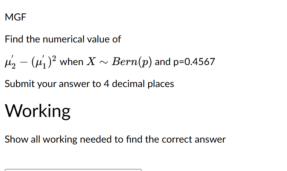
MGF & MOM

Moment Generating Functions

Estimating unknown parameters of a probability distribution using sample data. Given $X\sim \text{Bern}(p)$ We use the general formula: ${\mu }_k^{\prime }=\frac{d^k{M}_X(t)}{d{t}^k}{|}_{t=0}$ to find the k’th moment. taking the $k$-th derivative of the MGF with respect to $t$ and then plugging in $t=0$.

For example if our MGF is $M_X(t)=q+p{e}^t$ Then we would take the first derative $\frac{d}{dt}(q+p{e}^t)=0+p{e}^t$ Eval at t=0 $\frac{d{M}_X(t)}{dt}{|}_{t=0}=p{e}^0=p(1)=p$ mean ${\mu }_X$ is $p$ which is Parameter (Probability of Success)

Z-score + emnpirical

z-score (standard score) aka z-transformation

T.test Samples

t.test(x,y, 
       var.equal = TRUE, #equal variances ? (default false)
       conf.level = 0.80 #confidence interval
       )
...

• Take line below 95% conf interval, L = Left most value OPA

t_test_one_and_two_sample_Stats_Quiz

without t.test we need to do:

y <- c(3,4,5) #sample dataset
a = 0.2 #define alpha
n = length(y) #sample size
t <- qt(1-a/2,n-1) # critical t-value
 
mp = c(-1,1) #jsut to get both ends..
mean(y)+mp*t*sd(y)/sqrt(n) #final conf interval

Linear Combinations in Expected and Varience

• Finding E(#) plug mu in
• V(#) drop +b square entire thing (we always have to square all terms in V(#))!
  • if iid directly plug ${\sigma }^2$ into entire expr ^2, stats_linear_combo p2 Y=aX+b,L$