Stats_cheat_sheet_fina

t tests — make sure you know every detail of these

• including $var.equal=TRUE/FALSE$

When true: population variances are equal. Called Pooled $t$-Test. Use on fail 2 rej null hypothesis

t.test(group1_data, group2_data, 
       var.equal = TRUE, 
       alternative = "two.sided")

When false Welch $t$-Test. safer choice unless there is strong evidence for equal variances Use when reject null hypothesis from var.test. Same as above, but false.

NULL $H_0$ and Alternate hypotheses $H_a$

• $H_0$: Represents a statement of “no effect,” “no difference,” or “no relationship”
  • always includes an equality sign ($=$, $\le$, or $\ge$).
• $H_a$ what you’re trying to find.

t.test(Group\_A, Group\_B, alternative = "\text{less}")

Using data in R to create tests

Predictions

SLR:

$\hat{E}(Y|x_p)={\hat{Y}}_p={\hat{\beta }}_0+{\hat{\beta }}_1{x}_p$ - expected value of the response variable $Y$ for a specific value p of the predictor variable $x$ - mean response of the population when the predictor variable is fixed at $x_p$ -

• Least Squares estimates
  • Find values for the slope (${\hat{\beta }}_1$) and the intercept (${\hat{\beta }}_0$) that minimize Sum of Squared Errors (SSE) use

a = lm(y_data ~ x_data)
summary(a)

• ci confidence interval creation in r

# Find the 95% Confidence Intervals for the Intercept and Slope
confint(my_model, level = 0.95)

Use s20x package

MGF

Packages all raw moments of random variable $X$ into an expr. 2 ways to find ${\sigma }^2$ (vaience) and $\mu$ (mean). To find $r$-th raw moment, $E[X^r]$ take derative a@ 0 ${\text{M}}^{(r)}(0)=\frac{d^r}{d{t}^r}M(t){|}_{t=0}=E[X^r]$

• $\mu =E[X]=M^{\prime }(0)$
• Find ${\sigma }^2$ : calculated using the second and first raw moments:$Var(X)=E[X^2]-(E[X]{)}^2=M^{\prime \prime }(0)-[M^{\prime }(0){]}^2$

• Identify distributions

Gaps

$L=a_1{Y}_1+a_2{Y}_2+\cdot \cdot \cdot +a_n{Y}_n$ (or $l=a\_1Y\_1+...+a\_4Y\_4$ stuff)

• $E(L)$ (or $E(l)$)
• $V(L)$ (or $V(l)$)

Power

Probability of correctly rejecting $H_0$ when $H_a$ true aka $\text{Power}=1-\beta$

power_result <- power.t.test(
  n = 30,             # Sample size
  delta = 1,          # The true difference in means (Effect Size)
  sd = 2,             # Population standard deviation
  sig.level = 0.05,   # Significance level (alpha)
  type = "one.sample",# Type of t-test
  alternative = "two.sided" # Hypothesis direction
)

Calculate probabilities in R

LSE and varience

make predictions using the estimated regression line

• ${\hat{\beta }}_1=\frac{S{S}_{xy}}{S{S}_{xx}}$ LSE for slope
  • Sample estimate of the slope, calculated by dividing the sample covariance of $X$ and $Y$ (scaled by $n-1$) by the sample variance of $X$ (scaled by $n-1$).
  • defines the steepness of the estimated regression line
• $V({\hat{\beta }}_0)={\sigma }^2(\frac{{\sum }_{i=1}^n{x_i}^2}{nS{S}_{XX}})$ Varience of LSE for intercept $B_0$
  • calculate the Standard Error of ${\hat{\beta }}_0$, which is then used in the $t$-test for $H_0:{\beta }_0=0$ and the CI for ${\beta }_0$.

 my_model <- lm(y_data ~ x_data)
coefficients(my_model)
 
beta_0_hat <- coefficients(my_model)[1] # The Intercept
beta_1_hat <- coefficients(my_model)[2] # The Slope (x_data)

Show the estimators $\hat{\theta }$ are unbiased

unbiased if its expected value is equal to the true population parameter $\theta$ being estimated:

Find their variances etc

t-tests:

• Can you derive results by hand (P-values, t values, cis)

Perform tests using the three methods: CI, P values, RAR

Setup: We’re already given the output from t.test, and need to confirm the rest of the things Testing for population mean $\mu$:

$$\begin{array}{c}{H}_0:\mu =50\\ H_a:\mu \ne 50\end{array}$$

• Confidence interval:
  • Reject $H_0$ if the null value (${\mu }_0$) is not in CI

To get bounds:

estimate <- 7.9140
std_error <- 0.2471
t_critical <- 2.048
lower_bound <- estimate - t_critical * std_error
upper_bound <- estimate + t_critical * std_error
#which are our bounds..

• P-value:
  • Fail to Reject $H_0$ if the P-value $\ge \alpha$ from t.test
• Rejection/Acceptance Region (RAR):
  • Fail to Reject $H_0$ if the calculated test statistic ($t_{\text{calc}}$) falls into the acceptance region (i.e., $|t_{\text{calc}}|\le t_{\text{crit}}$).

# RAR example
alpha <- 0.05 df <- 28 # From the SLR summary example in the file 
t_critical <- qt(1 - alpha/2, df)
#then if t_calc is 3.0, and t_crit = 2, reject H_0

$t_{\text{calc}}=\frac{(\text{Estimate})-(\text{Null Value})}{\text{Standard Error of the Estimate}}$

• When use a $var.test$?
  • conduct two-sample independent $t$-test

Estimation:

• Max Lik: can you perform these calculations and proofs?
• Bootstrap — do you understand the code?

# Basic Bootstrap for a mean in R
n <- length(my_data)
B <- 10000 # Number of resamples
results <- numeric(B)
 
for(i in 1:B) {
  # Resample with replacement
  resample <- sample(my_data, size = n, replace = TRUE)
  results[i] <- mean(resample)
}
 
# Find the Bootstrap Confidence Interval
quantile(results, c(0.025, 0.975))

• Interval estimation: can you derive results that we did in class?

• Expected Value $E(L)$:
  • $E(\sum Y_i)=\sum E(Y_i)$
  • For Exponential data, $E(Y_i)=1/\lambda$, so $E(L)=n/\lambda$
• Variance $V(L)$:
  • Assuming independence, $V(\sum Y_i)=\sum V(Y_i)$
  • For Exponential data, $V(Y_i)=1/{\lambda }^2$, so $V(L)=n/{\lambda }^2$
• Distribution:
  • By the Central Limit Theorem, if $n$ is large, $L$ will be approximately Normal11.
  • $L\sim N(\frac{n}{\lambda },\frac{n}{{\lambda }^2})$

Regression:

#use
a= lm()
summary(a)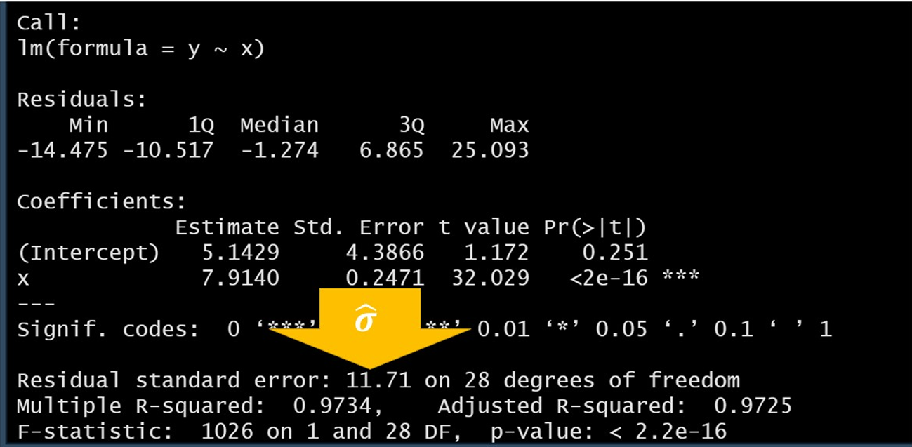

• ${\hat{\beta }}_0$ (Intercept) = 5.14…
• ${\hat{\beta }}_1$ (Slope) = 7.91..
• for SLR sample size = DOF +2 (30 in this case)
• Residual Standard Error ($\hat{\sigma }$): 11.71
• Multiple R-squared: 97.3% of the variation in $Y$ is explained by the linear relationship with $X$
• F-statistic: p-value is very small, we reject the null hypothesis
  • considered small if it is less than or equal to $\alpha$
• verify t-vales:
  • dividing the Estimate by the Std. Error in x row.
• Find t_crit:

t_crit <- qt(0.975, 28)# 28 = dfm 0.975  for 95% conf interval

Bootstrap and other R functions are shown in the labs

Be able to recognize options, default values and ellipses

All relevant Labs — especially tests, Max lik (lab 10) and labs 14-16 on regression