Stat_ch10 Notes (lab3) MSS TSS RSS

Statistic	Formula	Comparison
RSS	$\sum (y-\hat{y}{)}^2$	actual vs predicted
MSS	∑(y^−yˉ)2\sum (\hat{y} - \bar{y})^2	predicted vs mean
TSS	∑(y−yˉ)2\sum (y - \bar{y})^2	actual vs mean

# Residual Sum of Squares (RSS)

Info

• measure of how good the model approximates the data (measures model error)
• Residuals are the differences between the observed data values and the least squares regression line
• Calculated by: Residual = Observed – Predicted
• They represent the error!! (Sum of all the point to line distances)
• Graphically, residuals are the vertical distances between the observed values and the line

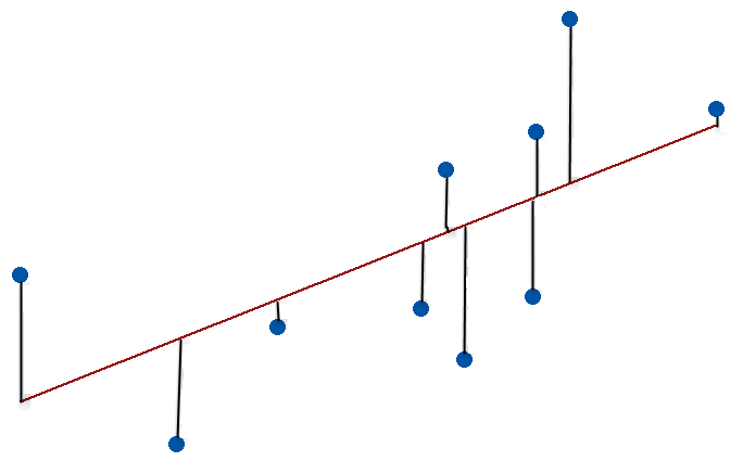(hence its the lines from pts to line)

Formula:

$$RSS=\sum _{i=1}^n{\left(y_i-{\hat{y}}_i\right)}^2$$

• $y_i$ = actual observed value of the response (dependent variable) at point $i$
• ${\hat{y}}_i$ = predicted value from the regression model

Code

Adding on Residual line segments to a plot

yhat = fitted(spruce.lm) #fitted: returns the predicted values of the dependent variable
segments(ddt$BHDiameter, #x_1
    	 ddt$Height, #x_1
    	 ddt$BHDiameter, #x_2
    	 yhat #y_2
    	 )
#segments esentially adds drawn line ontop of current graph, #so we have base pt to predicted point (line to point)

Direct residuals calculation

residuals(object..) #OR 
resid(...)
#extracts model residuals from objects returned by modeling functions

Ordinary Least Squares Regression

• method of constructing a good model
• Aka Line of best fit, minimizes the RSS

Code:

linear_reg = with(ddt, lm(y~x)) #to obtain a line (non graph), y~x is y related to x
#we can use abline(linear_reg) ontop of an existing plot to add this line on

Formula (not impt)

${\hat{y}}_i={\hat{\beta }}_0+{\hat{\beta }}_1{x}_i$

• $(y_i-{\hat{y}}_i)$ = residual (the error at point $i$)
• $(y_i-{\hat{y}}_i{)}^2$ = squared residual (penalizes larger errors more heavily)
• ${\sum }_{i=1}^n$ = summation across all data points

model sum of squares (MSS)

Same base formula:

$$RSS=\sum _{i=1}^n{\left(y_i-{\hat{y}}_i\right)}^2$$

But:

• $y_i=$ predicted value of the dependent variable
• $\widehat{y_i}=$ mean of the dependent variable

Code:

• Mean of Y versus X i.e. mean of Height vs BHDiameter, deviations of the fitted line from the mean height added. (MSS=model sum of squares)
• We didn’t include fitted line but its from OLSR code

segments(ddt$BHDiameter, #x_1
         mean(ddt$Height),  #y_1
         ddt$BHDiameter, 
         yhat, # yhat = fitted(linear_reg) # predicted value from the regression model
         )
abline(h=mean(ddt$Height)) # see abline 

total sum of squares (TSS)

NOTE

• RSS + MSS = TSS-  Sum of squared differences between the observed dependent variables and the overall mean
• $y_i=$ observed dependent variable
• $\widehat{y_i}=$ mean of the dependent variable

Code

Plot mean of Height versus BHDiameter + show total deviation line segments

segments(ddt$BHDiameter,#x_0
         ddt$Height, #y_0
         ddt$BHDiameter, #x_1
         mean(ddt$Height),#y_1, notice we dont use mean here!!
         )

Other code parts:

Scatter Plot w/ trend line etc

trendscatter(x~y,
    		 f=0.5, #smoothness of curve
    		  data=ddt)

Linear Model

lm(...)
#  carry out regression,
#ex: 
lm.D9 <- lm(weight ~ group)

Plot points

plot(Height~BHDiameter,bg="Blue",#circle colour
                pch=21, #circle width
                cex=1.2, #size of points
                ylim=c(0,1.1*max(Height)), #axis limits from 0 to 10% above the max Height
                xlim=c(0,1.1*max(BHDiameter))# vise versa
                )

Abline()..

abline(h = mean(y))  # horizontal line
abline(v = 5)                  # vertical line at x = 5
abline(a = 2, b = 0.5)         # line y = 2 + 0.5*x
abline(lm(y~x, data=ddt)) #takes LoBF in en plot ontop of cur graph  

See also

• stats_ch2 notes zscore chebvy chev
• Hub
• Stats_Lab4_notes